Creating Inputs for a Tide-Only FVCOM Simulation

This tutorial demonstrates how to take an SMS mesh file and generate all the basic input files required to run a tide-only FVCOM simulation using PyFVCOM2.

Overview

A tide-only FVCOM run requires:

1. Grid file (.dat) — the unstructured mesh

2. Open boundary file (obc.dat) — which nodes lie on the open boundary and their type

3. Depth file (optional, .dat) — bathymetry at each node

4. Coriolis file (.dat) — latitude used to compute the Coriolis parameter

5. Sigma coordinate file (sigma.dat) — the vertical layer distribution

6. OBC tidal elevation forcing file (.nc) — predicted tidal elevations at open boundary nodes

We start from an SMS .2dm mesh file for the North-West European shelf and work through each step, producing all the above files.

Prerequisites

• PyFVCOM2 installed with all dependencies

• TPXO tidal atlas data files

• An SMS .2dm mesh file with open boundary node strings defined

1. Import Required Libraries

import os
import numpy as np
import matplotlib.pyplot as plt
import matplotlib.tri as mtri
from datetime import datetime, timedelta

from pyfvcom2.grid import create_grid
from pyfvcom2.sigma import read_sigma_file, process_sigma_config
from pyfvcom2.tide import TideManager
from pyfvcom2.tide_reader import TPXOComplexHarmonicsReader, get_tpxo_complex_harmonics_names
from pyfvcom2.interpolation import TPXOInterpolator
from pyfvcom2.obc import OBCManager

/local1/data/scratch/jcl/miniconda/miniconda3/envs/pyfvcom2/lib/python3.11/site-packages/numpy/lib/_format_impl.py:838: VisibleDeprecationWarning: dtype(): align should be passed as Python or NumPy boolean but got `align=0`. Did you mean to pass a tuple to create a subarray type? (Deprecated NumPy 2.4)
  array = pickle.load(fp, **pickle_kwargs)

2. Configuration

Set all file paths and simulation parameters in one place.

data_dir = os.path.expanduser('~/data/pyfvcom2_doc')

# Input files
mesh_file   = f'{data_dir}/FVCOM_north_sea/nsea_v09.2dm'
sigma_file  = f'{data_dir}/FVCOM_north_sea/sigma_gen.dat'

# TPXO tidal atlas
tpxo_dir  = f'{data_dir}/TPXO/DATA/Atlas10v2'
constituents = ['M2', 'S2', 'K1', 'O1', 'N2', 'K2']
tpxo_h_files = {c: f'{tpxo_dir}/h_{c.lower()}_tpxo10_atlas_30_v2.nc' for c in constituents}
tpxo_bathy   = f'{tpxo_dir}/grid_tpxo10atlas_v2.nc'

# Output files
out_dir       = f'{data_dir}/FVCOM_north_sea/inputs'
os.makedirs(out_dir, exist_ok=True)

out_grid     = f'{out_dir}/nsea_grd.dat'
out_depth    = f'{out_dir}/nsea_dep.dat'
out_obc      = f'{out_dir}/nsea_obc.dat'
out_coriolis = f'{out_dir}/nsea_cor.dat'
out_sigma    = f'{out_dir}/sigma_gen.dat'
out_tides    = f'{out_dir}/nsea_tides_obc.nc'

# Simulation period
start_date = datetime(2025, 1,  1)
end_date   = datetime(2025, 1, 31)
dt         = timedelta(hours=1)
dates = [start_date + i * dt for i in range(int((end_date - start_date) / dt) + 1)]

print(f'Mesh file:       {mesh_file}')
print(f'Output dir:      {out_dir}')
print(f'Simulation:      {start_date} → {end_date}  ({len(dates)} time steps)')

Mesh file:       /users/modellers/jcl/data/pyfvcom2_doc/FVCOM_north_sea/nsea_v09.2dm
Output dir:      /users/modellers/jcl/data/pyfvcom2_doc/FVCOM_north_sea/inputs
Simulation:      2025-01-01 00:00:00 → 2025-01-31 00:00:00  (721 time steps)

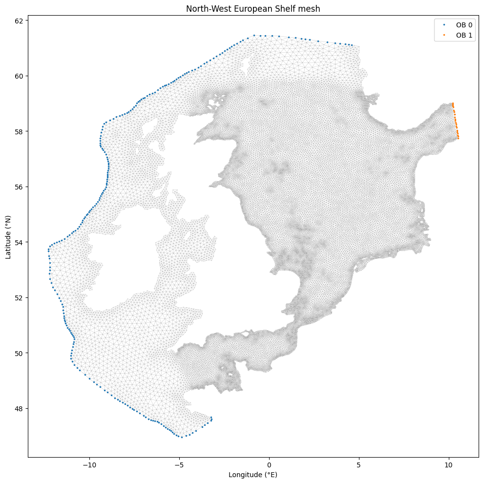
3. Load the Mesh

Read the SMS .2dm mesh and sigma file into a Grid object. The mesh uses geographic coordinates (longitude/latitude), so we set coordinate_system='geographic'. Open boundary node strings are embedded in the .2dm file, so no separate OBC file is needed at this stage.

grid = create_grid(
    mesh_file,
    mesh_type='sms',
    sigma_file=sigma_file,
    coordinate_system='geographic',
    nodestrings=True,
)

print(f'Nodes:             {grid.n_nodes}')
print(f'Elements:          {grid.n_elements}')
print(f'Sigma levels:      {grid.n_sigma_levels}')
print(f'Open boundaries:   {grid.n_open_boundaries}')
print(f'Longitude range:   {grid.lon_nodes.min():.2f} → {grid.lon_nodes.max():.2f}°E')
print(f'Latitude range:    {grid.lat_nodes.min():.2f} → {grid.lat_nodes.max():.2f}°N')
print(f'Depth range:       {grid.bathy_nodes.min():.1f} → {grid.bathy_nodes.max():.1f} m')

Nodes:             26522
Elements:          50719
Sigma levels:      25
Open boundaries:   2
Longitude range:   -12.28 → 10.53°E
Latitude range:    46.96 → 61.45°N
Depth range:       5.0 → 687.0 m

Visualise the mesh

Plot the mesh with open boundary nodes highlighted.

fig, ax = plt.subplots(figsize=(10, 10))
ax.triplot(grid.lon_nodes, grid.lat_nodes, grid.triangles, linewidth=0.2, color='0.6')

colors = plt.cm.tab10.colors
for i, ob in enumerate(grid.open_boundaries):
    ax.plot(grid.lon_nodes[ob.node_indices], grid.lat_nodes[ob.node_indices],
            '.', color=colors[i % len(colors)], markersize=3,
            label=f'OB {i}')

ax.set_xlabel('Longitude (°E)')
ax.set_ylabel('Latitude (°N)')
ax.set_title('North-West European Shelf mesh')
ax.legend()
plt.tight_layout()
plt.show()

4. Write the Grid and Depth Files

write_grid writes the FVCOM-format unstructured grid file. Passing depth_file also produces a separate bathymetry file (used with the GRID_DEPTH_FILE namelist option).

grid.write_grid(out_grid, coordinate_system='geographic', depth_file=out_depth)
print(f'Written: {out_grid}')
print(f'Written: {out_depth}')

Written: /users/modellers/jcl/data/pyfvcom2_doc/FVCOM_north_sea/inputs/nsea_grd.dat
Written: /users/modellers/jcl/data/pyfvcom2_doc/FVCOM_north_sea/inputs/nsea_dep.dat

5. Write the Open Boundary File

The obc.dat file lists each open boundary node with its 1-based index and boundary type. Type 1 is a simple tidal elevation boundary, which is what we need for a tide-only run.

grid.write_obc(out_obc)
print(f'Written: {out_obc}')

n_obc = sum(ob.nnodes for ob in grid.open_boundaries)
print(f'Total OBC nodes: {n_obc}')

Written: /users/modellers/jcl/data/pyfvcom2_doc/FVCOM_north_sea/inputs/nsea_obc.dat
Total OBC nodes: 255

6. Write the Coriolis File

The Coriolis file provides the latitude at each node, from which FVCOM computes the Coriolis parameter \(f = 2\Omega \sin(\phi)\).

grid.write_coriolis(out_coriolis, coordinate_system='geographic')
print(f'Written: {out_coriolis}')

Written: /users/modellers/jcl/data/pyfvcom2_doc/FVCOM_north_sea/inputs/nsea_cor.dat

7. Write the Sigma Coordinate File

The sigma file defines the vertical layer distribution. Here we simply copy the configuration that was read in with the grid — the sigma coordinate parameters are stored on the Grid object.

grid.write_sigma(out_sigma)
print(f'Written: {out_sigma}')
print(f'Sigma type: {grid.sigma_config.sigtype}')
print(f'Levels:     {grid.n_sigma_levels}')

Written: /users/modellers/jcl/data/pyfvcom2_doc/FVCOM_north_sea/inputs/sigma_gen.dat
Sigma type: generalized
Levels:     25

8. Generate OBC Tidal Elevation Forcing

For a tide-only run, FVCOM needs a time series of sea surface elevation at the open boundary nodes, constructed from tidal harmonics.

We use:

• TPXOComplexHarmonicsReader to read the TPXO atlas harmonic constituents

• TPXOInterpolator to interpolate harmonics onto the OBC node positions

• TideManager to reconstruct the tidal time series

• OBCManager to write the FVCOM OBC elevation forcing NetCDF file

8.1 Load TPXO harmonics

# Bounding box with a margin to ensure full coverage of the OBC nodes
bbox = (
    grid.lon_nodes.min() - 1.0, grid.lon_nodes.max() + 1.0,
    grid.lat_nodes.min() - 1.0, grid.lat_nodes.max() + 1.0,
)

h_reader   = TPXOComplexHarmonicsReader(tpxo_h_files)
h_var_names = get_tpxo_complex_harmonics_names('zeta')
h_harmonics = h_reader.read_harmonics(
    constituents, h_var_names,
    fill_land=True, bbox=bbox, bbox_margin=0.1
)
h_interpolator = TPXOInterpolator(h_harmonics)

print(f'Loaded {len(h_harmonics.constituents)} constituents: {h_harmonics.constituents}')

Loaded 6 constituents: ['M2', 'S2', 'K1', 'O1', 'N2', 'K2']

8.2 Build the TideManager and predict elevations

tide_manager = TideManager(constituents=constituents)
tide_manager.add_interpolator('zeta', h_interpolator)

obc_manager = OBCManager(grid)
obc_manager.set_dates(dates)
obc_manager.add_tidal_data(tide_manager)

print('Tidal predictions computed.')
print(f'  zeta shape: {obc_manager._zeta.shape}  (n_times × n_obc_nodes)')

prep/calcs ... prep/calcs ... prep/calcs ... prep/calcs ... prep/calcs ... prep/calcs ... prep/calcs ... prep/calcs ... prep/calcs ... prep/calcs ... prep/calcs ... prep/calcs ... done.
prep/calcs ... done.
done.done.done.

prep/calcs ... prep/calcs ... done.done.prep/calcs ...


done.prep/calcs ... done.prep/calcs ... prep/calcs ...
prep/calcs ...
prep/calcs ... done.
done.prep/calcs ...
done.prep/calcs ...
done.prep/calcs ...
prep/calcs ... done.
done.prep/calcs ... done.
done.prep/calcs ...

done.prep/calcs ... done.done.
prep/calcs ...
prep/calcs ...
prep/calcs ... done.prep/calcs ...
done.prep/calcs ... done.

done.prep/calcs ...
prep/calcs ... prep/calcs ... done.
prep/calcs ... done.
prep/calcs ... done.
done.done.prep/calcs ...

done.done.done.done.prep/calcs ...
prep/calcs ... done.



prep/calcs ... prep/calcs ... done.done.prep/calcs ... prep/calcs ... prep/calcs ...

done.prep/calcs ...
prep/calcs ... prep/calcs ... done.
prep/calcs ... done.
done.prep/calcs ...
prep/calcs ... done.done.
prep/calcs ... done.done.
done.
prep/calcs ...
prep/calcs ...
done.prep/calcs ... prep/calcs ...
prep/calcs ... done.
prep/calcs ... done.
prep/calcs ... done.
done.prep/calcs ...
done.prep/calcs ...
prep/calcs ... done.
done.prep/calcs ... done.

prep/calcs ... prep/calcs ... done.
done.
prep/calcs ... prep/calcs ... done.done.
done.done.done.prep/calcs ...


done.
prep/calcs ... prep/calcs ... prep/calcs ...
prep/calcs ... done.prep/calcs ... done.

prep/calcs ... prep/calcs ... done.done.

prep/calcs ... done.prep/calcs ... done.

prep/calcs ... done.done.prep/calcs ...

prep/calcs ... prep/calcs ... done.done.done.

done.prep/calcs ...

prep/calcs ... prep/calcs ... prep/calcs ... done.done.

prep/calcs ... prep/calcs ... done.
prep/calcs ... done.
prep/calcs ... done.done.
done.done.
done.prep/calcs ... prep/calcs ...

prep/calcs ... done.prep/calcs ...

done.prep/calcs ... done.

prep/calcs ... prep/calcs ... done.prep/calcs ...
prep/calcs ... done.done.done.

done.prep/calcs ... prep/calcs ...
prep/calcs ... done.

prep/calcs ... prep/calcs ... done.
prep/calcs ... done.done.
done.prep/calcs ...

prep/calcs ... done.
prep/calcs ... done.prep/calcs ...
prep/calcs ... done.
done.
done.prep/calcs ... done.prep/calcs ... done.done.done.

prep/calcs ... done.
done.

prep/calcs ...

prep/calcs ... prep/calcs ... prep/calcs ... prep/calcs ... prep/calcs ... done.
prep/calcs ... done.
done.prep/calcs ...
done.done.done.prep/calcs ...

done.

prep/calcs ... prep/calcs ... prep/calcs ... prep/calcs ... done.done.

prep/calcs ... prep/calcs ... done.
done.prep/calcs ...
prep/calcs ... done.done.done.
prep/calcs ...

prep/calcs ... prep/calcs ... done.
prep/calcs ... done.done.done.
done.


prep/calcs ... prep/calcs ... prep/calcs ... prep/calcs ... done.
done.prep/calcs ...
prep/calcs ... done.done.
done.
prep/calcs ... done.done.prep/calcs ...


prep/calcs ... prep/calcs ... prep/calcs ... done.done.done.
done.
done.prep/calcs ... prep/calcs ...


prep/calcs ... prep/calcs ... prep/calcs ... done.done.
prep/calcs ...
done.prep/calcs ...
done.prep/calcs ... done.

prep/calcs ... done.prep/calcs ...
done.
prep/calcs ... prep/calcs ... done.
done.done.prep/calcs ...

prep/calcs ... done.prep/calcs ... done.

done.prep/calcs ... prep/calcs ... done.

prep/calcs ... done.prep/calcs ...
done.prep/calcs ... done.

done.prep/calcs ... done.prep/calcs ... done.
prep/calcs ...
done.prep/calcs ...
prep/calcs ...
done.
prep/calcs ... prep/calcs ... done.
prep/calcs ... done.done.
done.

prep/calcs ... done.prep/calcs ...
prep/calcs ... prep/calcs ... done.
prep/calcs ... done.
done.done.
prep/calcs ... prep/calcs ...
done.prep/calcs ...
done.prep/calcs ...
done.prep/calcs ... done.

prep/calcs ... prep/calcs ... done.done.

done.prep/calcs ... prep/calcs ... done.

prep/calcs ... prep/calcs ... done.
prep/calcs ... done.done.
prep/calcs ...
done.done.done.
prep/calcs ... prep/calcs ... done.
done.prep/calcs ... done.


prep/calcs ... prep/calcs ... done.prep/calcs ...
prep/calcs ... done.
prep/calcs ...
prep/calcs ... done.
prep/calcs ... done.done.done.


prep/calcs ... prep/calcs ... prep/calcs ... done.done.
done.

prep/calcs ... done.done.prep/calcs ... prep/calcs ...

done.prep/calcs ... done.prep/calcs ...

done.prep/calcs ... prep/calcs ...
prep/calcs ... done.
prep/calcs ... done.
done.prep/calcs ...
prep/calcs ... done.done.done.

prep/calcs ...
done.prep/calcs ... prep/calcs ... done.
done.
prep/calcs ... prep/calcs ...
prep/calcs ... done.done.
done.prep/calcs ...
done.
prep/calcs ...
prep/calcs ... prep/calcs ... done.
done.done.
done.
prep/calcs ... prep/calcs ...
done.done.prep/calcs ... done.

prep/calcs ...
done.prep/calcs ... prep/calcs ... done.done.done.



prep/calcs ... done.
done.
done.prep/calcs ... done.
done.done.
done.
prep/calcs ... prep/calcs ...
prep/calcs ...
prep/calcs ... prep/calcs ... done.
prep/calcs ... done.
done.
prep/calcs ... done.done.

prep/calcs ... done.done.prep/calcs ...

prep/calcs ... prep/calcs ... done.done.

prep/calcs ... prep/calcs ... done.
prep/calcs ... done.done.done.


prep/calcs ... prep/calcs ... prep/calcs ... done.
prep/calcs ... done.done.

prep/calcs ... done.done.done.done.



prep/calcs ... prep/calcs ... prep/calcs ... done.done.

done.done.

Tidal predictions computed.
  zeta shape: (721, 255)  (n_times × n_obc_nodes)

8.3 Write the forcing file

obc_manager.create_forcing_file(
    out_tides,
    ncopts={'zlib': True, 'complevel': 4},
)
print(f'Written: {out_tides}')
print(f'File size: {os.path.getsize(out_tides) / 1024:.1f} kB')

Written: /users/modellers/jcl/data/pyfvcom2_doc/FVCOM_north_sea/inputs/nsea_tides_obc.nc
File size: 699.4 kB

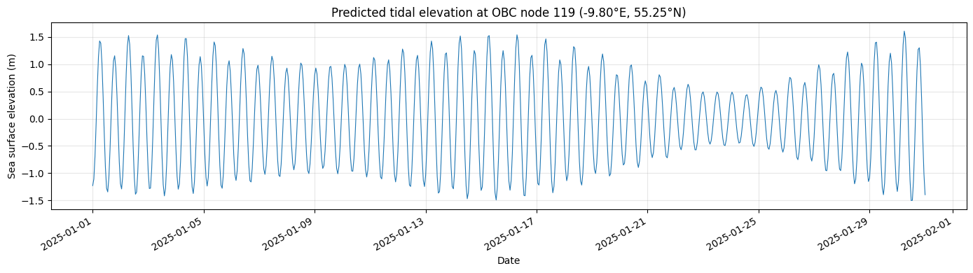
8.4 Visualise the predicted tides at a sample OBC node

# Pick the midpoint of the first open boundary for illustration
sample_idx = len(grid.open_boundaries[0].node_indices) // 2
sample_node = grid.open_boundaries[0].node_indices[sample_idx]
sample_lon = grid.lon_nodes[sample_node]
sample_lat = grid.lat_nodes[sample_node]

zeta_sample = obc_manager._zeta[:, sample_idx]

fig, ax = plt.subplots(figsize=(14, 4))
ax.plot(dates, zeta_sample, linewidth=0.8)
ax.set_xlabel('Date')
ax.set_ylabel('Sea surface elevation (m)')
ax.set_title(f'Predicted tidal elevation at OBC node {sample_node} '
             f'({sample_lon:.2f}°E, {sample_lat:.2f}°N)')
ax.grid(True, alpha=0.3)
fig.autofmt_xdate()
plt.tight_layout()
plt.show()

9. Summary

The following files have been written to out_dir and are ready to be referenced in the FVCOM namelist for a tide-only run:

File	Namelist key
nsea_grd.dat	GRID_FILE
nsea_dep.dat	GRID_DEPTH_FILE
nsea_obc.dat	OBC_NODE_LIST
nsea_cor.dat	CORIOLIS_FILE
sigma_gen.dat	SIGMA_PARAMETER_FILE
nsea_tides_obc.nc	TIDAL_FORCING_FILE

Once FVCOM has run in tide-only mode and produced output, you can use PyFVCOM2’s harmonic analysis tools to extract tidal constituents and build a harmonics file for use in a full baroclinic simulation with nest forcing.