Visualising the Nest Forcing Ramp

When an FVCOM model is started from rest, applying full boundary forcing immediately can cause a numerical shock. NestManager.apply_ramp() addresses this by smoothly blending each forcing variable from a calm initial state up to its full value. Three ramp shapes are available via the ramp_type argument:

ramp_type	Formula	Smoothness	Reaches full amplitude
'cosine' (default)	\(\frac{1}{2}\!\left(1 - \cos\!\left(\frac{\pi t}{T}\right)\right)\)	\(C^1\) at both ends	Exactly at \(t = T\)
'tanh'	\(\tanh\!\left(\frac{t}{T}\right)\)	\(C^\infty\) everywhere	Asymptotic (~76 % at \(t=T\), ~99.5 % at \(t=3T\))
'linear'	\(\min\!\left(\frac{t}{T},\,1\right)\)	\(C^0\) (kinked)	Exactly at \(t = T\)

For all types, the forcing at each time step is:

\[f_{\text{ramped}}(t) = f_0 \,(1 - \text{ramp}(t)) + f(t)\,\text{ramp}(t)\]

where \(f_0\) is the initial value (zero for velocities and zeta; user-supplied for temperature and salinity).

This notebook demonstrates the effect of apply_ramp() on synthetic forcing data, without requiring real CMEMS or grid files.

1. Imports

import warnings
import numpy as np
import matplotlib.pyplot as plt
import matplotlib.ticker as ticker
from datetime import datetime, timedelta

# Suppress a NumPy 2.4 deprecation warning that arises when loading .npy files
# saved with older NumPy versions (align stored as int 0 rather than bool).
warnings.filterwarnings(
    'ignore',
    message=r'dtype\(\): align should be passed as Python or NumPy boolean',
    category=np.exceptions.VisibleDeprecationWarning,
)

2. Ramp Shape

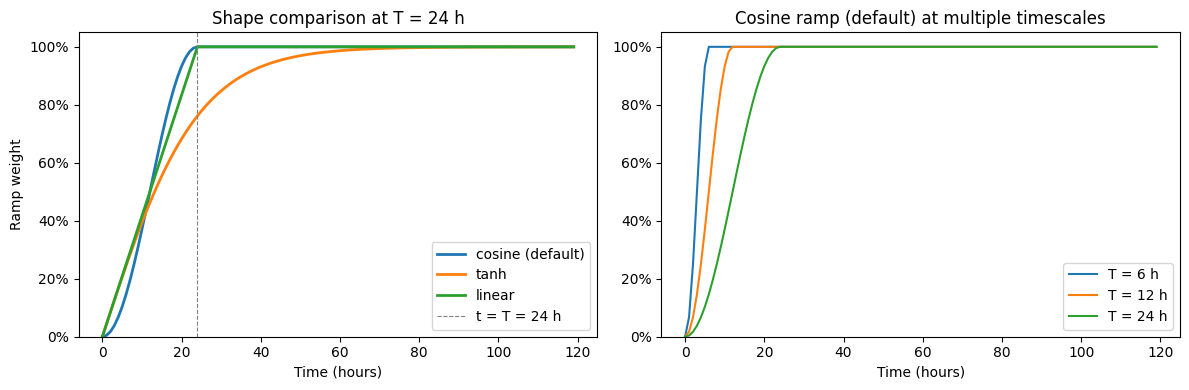
The three ramp types have different smoothness and endpoint properties. The left panel compares all three at the same ramp_length (T = 24 h). The right panel shows the cosine default at several timescales.

# Simulation period: 5 days at hourly resolution
start = datetime(2025, 6, 14)
n_hours = 5 * 24
dates = [start + timedelta(hours=h) for h in range(n_hours)]
t_sec = np.array([(d - dates[0]).total_seconds() for d in dates])
t_hours = t_sec / 3600

T_sec = 24 * 3600   # ramp_length for the shape comparison
ramp_cosine = np.where(t_sec >= T_sec, 1.0, 0.5 * (1 - np.cos(np.pi * t_sec / T_sec)))
ramp_tanh   = np.tanh(t_sec / T_sec)
ramp_linear = np.minimum(t_sec / T_sec, 1.0)

ramp_lengths_hours = [6, 12, 24]

fig, axes = plt.subplots(1, 2, figsize=(12, 4))

# Left: shape comparison at T = 24 h
axes[0].plot(t_hours, ramp_cosine, label='cosine (default)', color='tab:blue',   lw=2)
axes[0].plot(t_hours, ramp_tanh,   label='tanh',             color='tab:orange', lw=2)
axes[0].plot(t_hours, ramp_linear, label='linear',           color='tab:green',  lw=2)
axes[0].axvline(24, color='grey', lw=0.8, ls='--', label='t = T = 24 h')
axes[0].set_xlabel('Time (hours)')
axes[0].set_ylabel('Ramp weight')
axes[0].set_title('Shape comparison at T = 24 h')
axes[0].legend()
axes[0].set_ylim(0, 1.05)
axes[0].yaxis.set_major_formatter(ticker.PercentFormatter(xmax=1))

# Right: cosine (default) at multiple timescales
for T_h in ramp_lengths_hours:
    T_s = T_h * 3600
    ramp_c = np.where(t_sec >= T_s, 1.0, 0.5 * (1 - np.cos(np.pi * t_sec / T_s)))
    axes[1].plot(t_hours, ramp_c, label=f'T = {T_h} h')
axes[1].set_xlabel('Time (hours)')
axes[1].set_title('Cosine ramp (default) at multiple timescales')
axes[1].legend()
axes[1].set_ylim(0, 1.05)
axes[1].yaxis.set_major_formatter(ticker.PercentFormatter(xmax=1))

fig.tight_layout()
plt.show()

3. Synthetic Forcing Data

We generate simple synthetic time series to stand in for real forcing variables across a small number of points. The forcing is kept deliberately simple so the effect of the ramp is obvious:

Variable	Shape	Synthetic signal
zeta	(time, nodes)	constant + small diurnal oscillation
u, v	(time, depth, elements)	depth-varying sinusoid
temp	(time, depth, nodes)	realistic stratified profile
salinity	(time, depth, nodes)	realistic stratified profile

rng = np.random.default_rng(42)

n_times    = n_hours
n_nodes    = 20
n_elements = 12
n_sigma    = 10   # sigma layers

# --- zeta: constant offset + diurnal tide, shape (time, nodes) ---
omega_M2 = 2 * np.pi / (12.42 * 3600)   # M2 tidal frequency
zeta_amp  = 1.5 + 0.5 * rng.random(n_nodes)   # node-varying amplitude (m)
zeta = (zeta_amp[np.newaxis, :]
        * np.sin(omega_M2 * t_sec[:, np.newaxis]))

# --- u, v: depth-varying velocity, shape (time, sigma, elements) ---
depth_profile = np.linspace(1.0, 0.3, n_sigma)   # surface→bed shear
u_amp = 0.3 + 0.1 * rng.random(n_elements)
v_amp = 0.2 + 0.1 * rng.random(n_elements)
u = (u_amp[np.newaxis, np.newaxis, :]
     * depth_profile[np.newaxis, :, np.newaxis]
     * np.sin(omega_M2 * t_sec[:, np.newaxis, np.newaxis]))
v = (v_amp[np.newaxis, np.newaxis, :]
     * depth_profile[np.newaxis, :, np.newaxis]
     * np.cos(omega_M2 * t_sec[:, np.newaxis, np.newaxis]))

# --- temp: stratified profile, shape (time, sigma, nodes) ---
temp_surface = 15.0 + 0.5 * rng.random(n_nodes)
temp_bottom  =  9.0 + 0.2 * rng.random(n_nodes)
temp_profile = np.linspace(0, 1, n_sigma)[:, np.newaxis]   # 0=surface, 1=bottom
temp = (temp_surface[np.newaxis, np.newaxis, :]
        + temp_profile[np.newaxis, :, :]
        * (temp_bottom - temp_surface)[np.newaxis, np.newaxis, :])
temp = np.broadcast_to(temp, (n_times, n_sigma, n_nodes)).copy()

# --- salinity: stratified profile, shape (time, sigma, nodes) ---
sal_surface = 32.0 + 0.3 * rng.random(n_nodes)
sal_bottom  = 35.0 + 0.1 * rng.random(n_nodes)
salinity = (sal_surface[np.newaxis, np.newaxis, :]
            + temp_profile[np.newaxis, :, :]
            * (sal_bottom - sal_surface)[np.newaxis, np.newaxis, :])
salinity = np.broadcast_to(salinity, (n_times, n_sigma, n_nodes)).copy()

print('Synthetic data shapes:')
for name, arr in [('zeta', zeta), ('u', u), ('v', v),
                  ('temp', temp), ('salinity', salinity)]:
    print(f'  {name:10s}: {arr.shape}')

Synthetic data shapes:
  zeta      : (120, 20)
  u         : (120, 10, 12)
  v         : (120, 10, 12)
  temp      : (120, 10, 20)
  salinity  : (120, 10, 20)

4. Apply the Ramp

We replicate what NestManager.apply_ramp() does internally, calling NestManager._build_ramp and NestManager._apply_ramp_to_array directly. We generate four variants — all three types at T = 24 h, plus the default cosine at T = 6 h — to compare their effect on the forcing variables.

from pyfvcom2.nest import NestManager

def apply_ramp_to_data(forcing, ramp_length_sec, t_sec, ramp_type='cosine', initial_ts=None):
    """Apply a ramp to a dict of forcing arrays.

    Returns a new dict of ramped copies; the originals are unchanged.
    """
    ramp = NestManager._build_ramp(t_sec, ramp_length_sec, ramp_type)
    result = {}
    for var, data in forcing.items():
        if var in ('u', 'v', 'zeta'):
            init = 0.0
        elif var == 'temp' and initial_ts is not None:
            init = initial_ts[0]
        elif var == 'salinity' and initial_ts is not None:
            init = initial_ts[1]
        else:
            result[var] = data.copy()
            continue
        result[var] = NestManager._apply_ramp_to_array(data, ramp, init)
    return result

# Nominal initial T/S values (climatological or model background)
initial_ts = [10.0, 34.5]   # °C, PSU

forcing_raw = dict(zeta=zeta, u=u, v=v, temp=temp, salinity=salinity)

cosine_6h  = apply_ramp_to_data(forcing_raw,  6 * 3600, t_sec, ramp_type='cosine', initial_ts=initial_ts)
cosine_24h = apply_ramp_to_data(forcing_raw, 24 * 3600, t_sec, ramp_type='cosine', initial_ts=initial_ts)
tanh_24h   = apply_ramp_to_data(forcing_raw, 24 * 3600, t_sec, ramp_type='tanh',   initial_ts=initial_ts)
linear_24h = apply_ramp_to_data(forcing_raw, 24 * 3600, t_sec, ramp_type='linear', initial_ts=initial_ts)

print('Variants prepared: cosine T=6h, cosine T=24h, tanh T=24h, linear T=24h')

Variants prepared: cosine T=6h, cosine T=24h, tanh T=24h, linear T=24h

5. Visualisation

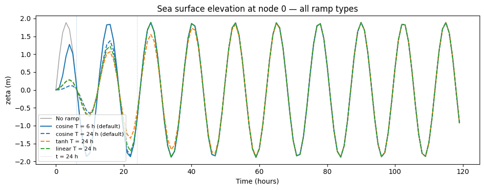
5a. Sea Surface Elevation (zeta) at a single node

All four variants are shown together, making it easy to compare the ramp shapes and timescales. Note that for tanh at T = 24 h the forcing has only reached ~76 % at t = 24 h, whereas both cosine and linear are at full amplitude by then.

node_idx = 0   # representative node

fig, ax = plt.subplots(figsize=(10, 4))
ax.plot(t_hours, forcing_raw['zeta'][:, node_idx],
        color='black', lw=1.2, label='No ramp', alpha=0.35)
ax.plot(t_hours, cosine_6h['zeta'][:, node_idx],
        color='tab:blue', lw=1.5, ls='-',  label='cosine T = 6 h (default)')
ax.plot(t_hours, cosine_24h['zeta'][:, node_idx],
        color='tab:blue', lw=1.5, ls='--', label='cosine T = 24 h (default)')
ax.plot(t_hours, tanh_24h['zeta'][:, node_idx],
        color='tab:orange', lw=1.5, ls='--', label='tanh T = 24 h')
ax.plot(t_hours, linear_24h['zeta'][:, node_idx],
        color='tab:green', lw=1.5, ls='--', label='linear T = 24 h')

ax.axvline( 6, color='tab:blue', lw=0.8, ls=':', alpha=0.5)
ax.axvline(24, color='grey',     lw=0.8, ls=':', alpha=0.5, label='t = 24 h')

ax.set_xlabel('Time (hours)')
ax.set_ylabel('zeta (m)')
ax.set_title(f'Sea surface elevation at node {node_idx} — all ramp types')
ax.legend(fontsize=8)
fig.tight_layout()
plt.show()

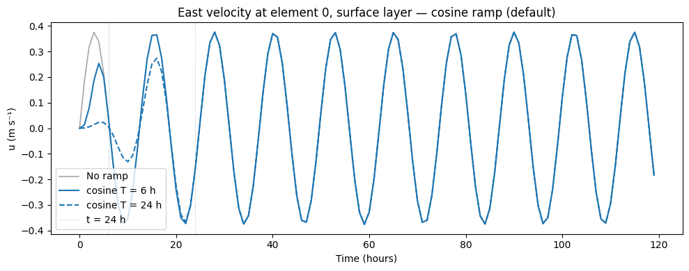
5b. Surface velocity (u) at a single element

The velocity is 3-D (time, sigma, element). Here we pick the surface layer.

elem_idx   = 0   # representative element
sigma_surf = 0   # surface sigma layer

fig, ax = plt.subplots(figsize=(10, 4))
ax.plot(t_hours, forcing_raw['u'][:, sigma_surf, elem_idx],
        color='black', lw=1.2, label='No ramp', alpha=0.35)
ax.plot(t_hours, cosine_6h['u'][:, sigma_surf, elem_idx],
        color='tab:blue', lw=1.5, ls='-',  label='cosine T = 6 h')
ax.plot(t_hours, cosine_24h['u'][:, sigma_surf, elem_idx],
        color='tab:blue', lw=1.5, ls='--', label='cosine T = 24 h')

ax.axvline( 6, color='tab:blue', lw=0.8, ls=':', alpha=0.5)
ax.axvline(24, color='grey',     lw=0.8, ls=':', alpha=0.5, label='t = 24 h')

ax.set_xlabel('Time (hours)')
ax.set_ylabel('u (m s⁻¹)')
ax.set_title(f'East velocity at element {elem_idx}, surface layer — cosine ramp (default)')
ax.legend()
fig.tight_layout()
plt.show()

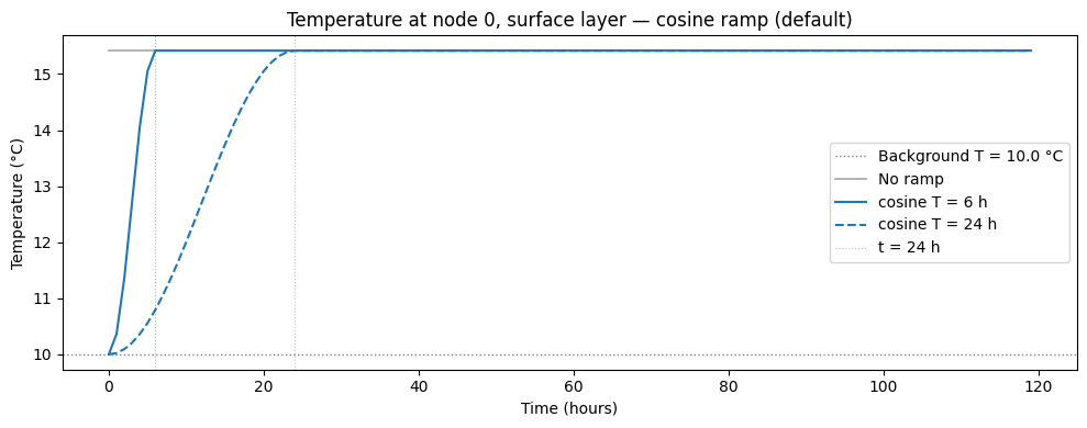
5c. Temperature ramp from an initial background value

Temperature (and salinity) are ramped from a user-supplied background state rather than from zero. Here we use an initial temperature of 10 °C and show the surface layer at one node.

node_idx   = 0
sigma_surf = 0
T0_temp    = initial_ts[0]   # 10 °C background

fig, ax = plt.subplots(figsize=(10, 4))
ax.axhline(T0_temp, color='grey', lw=1.0, ls=':', label=f'Background T = {T0_temp} °C')
ax.plot(t_hours, forcing_raw['temp'][:, sigma_surf, node_idx],
        color='black', lw=1.2, label='No ramp', alpha=0.35)
ax.plot(t_hours, cosine_6h['temp'][:, sigma_surf, node_idx],
        color='tab:blue', lw=1.5, ls='-',  label='cosine T = 6 h')
ax.plot(t_hours, cosine_24h['temp'][:, sigma_surf, node_idx],
        color='tab:blue', lw=1.5, ls='--', label='cosine T = 24 h')

ax.axvline( 6, color='tab:blue', lw=0.8, ls=':', alpha=0.5)
ax.axvline(24, color='grey',     lw=0.8, ls=':', alpha=0.5, label='t = 24 h')

ax.set_xlabel('Time (hours)')
ax.set_ylabel('Temperature (°C)')
ax.set_title(f'Temperature at node {node_idx}, surface layer — cosine ramp (default)')
ax.legend()
fig.tight_layout()
plt.show()

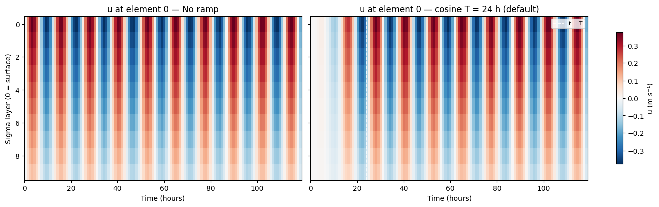
5d. Depth–time Hovmöller: velocity with and without ramp

This panel shows how the ramp suppresses velocity at all depths during spin-up, not just at the surface.

elem_idx = 0

u_raw_hov      = forcing_raw['u'][:, :, elem_idx].T   # (sigma, time)
u_cosine24_hov = cosine_24h['u'][:, :, elem_idx].T

vmax = np.abs(u_raw_hov).max()

fig, axes = plt.subplots(1, 2, figsize=(13, 4), sharey=True,
                         constrained_layout=True)
kw = dict(aspect='auto', origin='upper',
          extent=[0, t_hours[-1], n_sigma - 0.5, -0.5],
          vmin=-vmax, vmax=vmax, cmap='RdBu_r')

im0 = axes[0].imshow(u_raw_hov,      **kw)
im1 = axes[1].imshow(u_cosine24_hov, **kw)

for ax, title in zip(axes, ['No ramp', 'cosine T = 24 h (default)']):
    ax.set_xlabel('Time (hours)')
    ax.set_title(f'u at element {elem_idx} — {title}')

axes[0].set_ylabel('Sigma layer (0 = surface)')
axes[1].axvline(24, color='white', lw=1.2, ls='--', label='t = T')
axes[1].legend(loc='upper right', fontsize=8)

fig.colorbar(im0, ax=axes, label='u (m s⁻¹)', shrink=0.8)
plt.show()

6. Summary

NestManager.apply_ramp() supports three ramp shapes via the ramp_type argument:

ramp_type	Smoothness	Reaches full amplitude	Best suited for
'cosine' (default)	\(C^1\) at both ends	Exactly at \(t = T\)	Most cases — smooth, intuitive duration
'tanh'	\(C^\infty\) everywhere	Asymptotic	Very energetic boundaries where maximum smoothness is needed
'linear'	\(C^0\) (kinked at \(t=0\) and \(t=T\))	Exactly at \(t = T\)	Mild boundaries where simplicity is preferred

Key points:

• Velocities and zeta always start from zero and grow towards the full forcing value.

• Temperature and salinity start from a user-supplied background value (e.g. a model restart or climatological mean) and relax to the boundary forcing.

• For 'cosine' and 'linear', ramp_length means the spin-up is complete at \(t = T\). For 'tanh', it is a timescale: the spin-up is effectively complete at \(t \approx 3T\).

• A shorter ramp_length produces a steeper spin-up; a longer one is smoother but delays the model reaching full forcing.

A typical choice is ramp_length between 6 and 24 hours for an hourly-forced coastal model, depending on how energetic the open boundary is.