Bathymetry Smoothing
In sigma-coordinate ocean models such as FVCOM, sharp changes in bathymetry between adjacent elements can introduce spurious pressure gradient errors. The severity of this effect is quantified by the Haney r-factor:
where \(h_i\) and \(h_j\) are the mean depths of two adjacent elements. Values of \(r > 0.2\) are commonly associated with significant pressure gradient errors. FVCOM is generally less sensitive to this than finite-difference sigma-coordinate models, but pre-smoothing the bathymetry in regions with steep gradients is good practice.
PyFVCOM2 provides the GlobalBathymetrySmoother, which applies one or more passes of a node→centroid→node ping-pong interpolation across the entire mesh. Each pass is equivalent to a single Laplacian smoothing step and reduces sharp depth gradients uniformly.
Cold-start only. Smoothing changes the physical depth at every sigma level. Applying it after generating a restart file would produce an internally inconsistent hot start. Always smooth before generating forcing or restart files.
What this notebook covers
Load the Tamar estuary grid and visualise the mesh
Compute the r-factor distribution on the raw bathymetry
Apply the
GlobalBathymetrySmootherand compareWrite the smoothed grid to file
1. Imports and setup
[1]:
import copy
import os

import numpy as np
import matplotlib.pyplot as plt
import matplotlib.tri as mtri
import matplotlib.colors as mcolors
from matplotlib.patches import Rectangle

from pyfvcom2.grid import create_grid
from pyfvcom2.bathy_smoother import GlobalBathymetrySmoother
/local1/data/scratch/jcl/miniconda/miniconda3/envs/pyfvcom2/lib/python3.11/site-packages/numpy/lib/_format_impl.py:838: VisibleDeprecationWarning: dtype(): align should be passed as Python or NumPy boolean but got `align=0`. Did you mean to pass a tuple to create a subarray type? (Deprecated NumPy 2.4)
  array = pickle.load(fp, **pickle_kwargs)
[2]:
data_dir = os.path.expanduser('~/data/pyfvcom2_doc/FVCOM_tamar_estuary')

grid_file  = f'{data_dir}/tamar_v2_grd.dat'
obc_file   = f'{data_dir}/tamar_v2_obc.dat'
sigma_file = f'{data_dir}/sigma_gen.dat'

print(f'Grid:  {grid_file}')
print(f'OBC:   {obc_file}')
print(f'Sigma: {sigma_file}')
Grid:  /users/modellers/jcl/data/pyfvcom2_doc/FVCOM_tamar_estuary/tamar_v2_grd.dat
OBC:   /users/modellers/jcl/data/pyfvcom2_doc/FVCOM_tamar_estuary/tamar_v2_obc.dat
Sigma: /users/modellers/jcl/data/pyfvcom2_doc/FVCOM_tamar_estuary/sigma_gen.dat
2. Load the grid and visualise the mesh
[3]:
grid = create_grid(
    grid_file=grid_file,
    mesh_type='fvcom',
    sigma_file=sigma_file,
    coordinate_system='cartesian',
    obc_filename=obc_file,
    epsg_code='32630',
)

print(f'Nodes:    {grid.n_nodes:,}')
print(f'Elements: {grid.n_elements:,}')
print(f'Depth range: {grid.bathy_nodes.min():.1f} – {grid.bathy_nodes.max():.1f} m')
Nodes:    39,910
Elements: 75,400
Depth range: -6.6 – 80.3 m
[4]:
# ── Identify exterior boundary edges ──────────────────────────────────────
# An edge is a boundary edge if it belongs to exactly one element.
tris = grid.triangles
all_edges = np.vstack([
    np.column_stack([np.minimum(tris[:, 0], tris[:, 1]),
                     np.maximum(tris[:, 0], tris[:, 1])]),
    np.column_stack([np.minimum(tris[:, 1], tris[:, 2]),
                     np.maximum(tris[:, 1], tris[:, 2])]),
    np.column_stack([np.minimum(tris[:, 2], tris[:, 0]),
                     np.maximum(tris[:, 2], tris[:, 0])]),
])
unique_edges, counts = np.unique(all_edges, axis=0, return_counts=True)
bdy_edges = unique_edges[counts == 1]           # shape (n_bdy_edges, 2)

# Classify boundary edges as open-boundary or land
obc_node_arr = np.concatenate([obc.node_indices for obc in grid.open_boundaries])
is_obc_edge = np.isin(bdy_edges[:, 0], obc_node_arr) & np.isin(bdy_edges[:, 1], obc_node_arr)
land_edges = bdy_edges[~is_obc_edge]

# Efficient nan-separated arrays for plotting (one plot() call per segment type)
def _edge_lines(edges, lon, lat):
    out_x = np.empty(len(edges) * 3); out_x[2::3] = np.nan
    out_y = np.empty(len(edges) * 3); out_y[2::3] = np.nan
    out_x[0::3] = lon[edges[:, 0]]; out_x[1::3] = lon[edges[:, 1]]
    out_y[0::3] = lat[edges[:, 0]]; out_y[1::3] = lat[edges[:, 1]]
    return out_x, out_y

land_x, land_y = _edge_lines(land_edges, grid.lon_nodes, grid.lat_nodes)

# ── Figure layout ─────────────────────────────────────────────────────────
fig, ax = plt.subplots(figsize=(10, 8))

triang_geo = mtri.Triangulation(grid.lon_nodes, grid.lat_nodes, grid.triangles)

# Shaded bathymetry (alpha keeps grid lines visible through the fill)
tcf = ax.tricontourf(triang_geo, grid.bathy_nodes, levels=40, cmap='Blues', alpha=0.65)
fig.colorbar(tcf, ax=ax, label='Depth (m)', shrink=0.65, pad=0.02)

# Mesh grid lines
ax.triplot(triang_geo, color='0.35', linewidth=0.12, alpha=0.55)

# Land boundary
ax.plot(land_x, land_y, '-', color='#2d2d2d', linewidth=0.7, label='Land boundary')

# Open boundary segments (one colour per section)
obc_palette = ['#e74c3c', '#e67e22', '#8e44ad']
for i, obc in enumerate(grid.open_boundaries):
    ni = obc.node_indices
    col = obc_palette[i % len(obc_palette)]
    ax.plot(grid.lon_nodes[ni], grid.lat_nodes[ni], '-', color=col, linewidth=2.0,
            label=f'Open boundary (ID: {obc.bdy_id})')

ax.set_xlabel('Longitude')
ax.set_ylabel('Latitude')
ax.set_title('Tamar Estuary FVCOM Grid', fontsize=13)
ax.legend(loc='upper right', fontsize=8, framealpha=0.8)

# ── Plymouth Sound inset ──────────────────────────────────────────────────
# Approximate bounding box for Plymouth Sound / lower Tamar estuary
ps_lon = (-4.28, -4.00)
ps_lat = (50.30, 50.44)

ax_ins = ax.inset_axes([0.02, 0.02, 0.42, 0.38])

ax_ins.tricontourf(triang_geo, grid.bathy_nodes, levels=40, cmap='Blues', alpha=0.65)
ax_ins.triplot(triang_geo, color='0.35', linewidth=0.2, alpha=0.55)
ax_ins.plot(land_x, land_y, '-', color='#2d2d2d', linewidth=0.9)
for i, obc in enumerate(grid.open_boundaries):
    ni = obc.node_indices
    ax_ins.plot(grid.lon_nodes[ni], grid.lat_nodes[ni], '-',
                color=obc_palette[i % len(obc_palette)], linewidth=2.0)

ax_ins.set_xlim(*ps_lon)
ax_ins.set_ylim(*ps_lat)
ax_ins.set_xticks([])
ax_ins.set_yticks([])
ax_ins.set_title('Plymouth Sound', fontsize=9)
ax_ins.tick_params(labelsize=7)

# Rectangle on main plot showing the inset extent
rect = Rectangle((ps_lon[0], ps_lat[0]),
                 ps_lon[1] - ps_lon[0], ps_lat[1] - ps_lat[0],
                 linewidth=1.5, edgecolor='limegreen', facecolor='none')
ax.add_patch(rect)

plt.tight_layout()
plt.show()

print(f'Open boundaries: {grid.n_open_boundaries}')
for obc in grid.open_boundaries:
    print(f'  OB {obc.bdy_id} has {obc.nnodes} nodes')
print(f'Land boundary edges: {len(land_edges):,}')
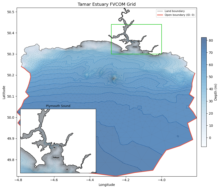
Open boundaries: 1
  OB 0 has 45 nodes
Land boundary edges: 4,388
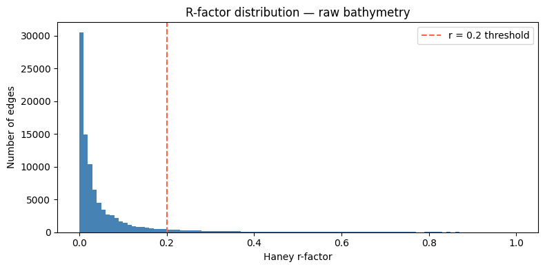
3. R-factor distribution on the raw bathymetry
The GlobalBathymetrySmoother exposes an r_factor() method that computes the Haney r-factor for every inter-element edge without modifying the grid. We use this as a diagnostic on the original bathymetry before any smoothing.
[5]:
smoother = GlobalBathymetrySmoother(passes=3)

r_raw = smoother.r_factor(grid)

n_total   = len(r_raw)
n_wet     = int((~np.isnan(r_raw)).sum())
n_masked  = n_total - n_wet

print(f'Depth range: {grid.bathy_nodes.min():.2f} to {grid.bathy_nodes.max():.1f} m')
print()
print(f'Total inter-element edges:  {n_total:,}')
print(f'  Submerged (evaluated):    {n_wet:,}')
print(f'  Intertidal (masked):      {n_masked:,}')
print()
print(f'Max r-factor:       {np.nanmax(r_raw):.4f}')
print(f'Mean r-factor:      {np.nanmean(r_raw):.4f}')
n_bad = int((r_raw > 0.2).sum())
print(f'Edges with r > 0.2: {n_bad:,} ({100*n_bad/n_wet:.1f}% of submerged edges)')
Depth range: -6.56 to 80.3 m

Total inter-element edges:  110,884
  Submerged (evaluated):    94,617
  Intertidal (masked):      16,267

Max r-factor:       1.0000
Mean r-factor:      0.0618
Edges with r > 0.2: 7,053 (7.5% of submerged edges)
[6]:
fig, ax = plt.subplots(figsize=(8, 4))
ax.hist(r_raw, bins=100, color='steelblue', edgecolor='none')
ax.axvline(0.2, color='tomato', linestyle='--', label='r = 0.2 threshold')
ax.set_xlabel('Haney r-factor')
ax.set_ylabel('Number of edges')
ax.set_title('R-factor distribution — raw bathymetry')
ax.legend()
plt.tight_layout()
plt.show()
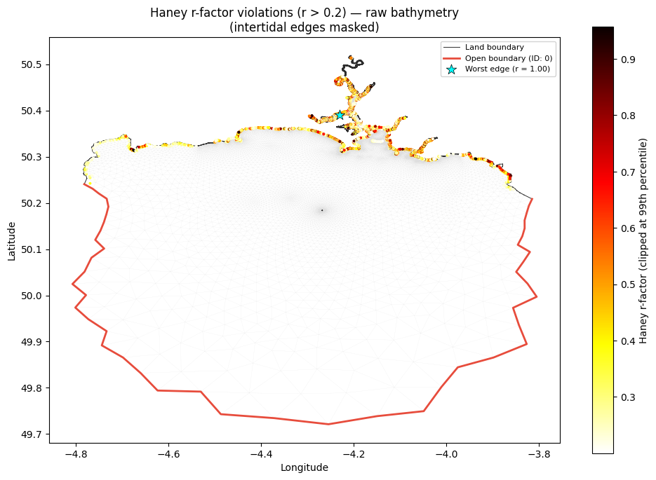
[7]:
# ── Shared-edge midpoints in geographic coordinates ─────────────────────
# Reuses triang_geo, land_x/y, obc_palette from the mesh visualisation cell.
h_nodes = grid.bathy_nodes
triangles = grid.triangles

edge_to_elem: dict = {}
edge_node_pairs: list = []

for ei, tri in enumerate(triangles):
    for a, b in ((tri[0], tri[1]), (tri[1], tri[2]), (tri[2], tri[0])):
        key = frozenset((int(a), int(b)))
        if key in edge_to_elem:
            edge_node_pairs.append((int(a), int(b)))
        else:
            edge_to_elem[key] = ei

edge_node_pairs = np.array(edge_node_pairs, dtype=np.intp)
edge_mlon = (grid.lon_nodes[edge_node_pairs[:, 0]] + grid.lon_nodes[edge_node_pairs[:, 1]]) / 2
edge_mlat = (grid.lat_nodes[edge_node_pairs[:, 0]] + grid.lat_nodes[edge_node_pairs[:, 1]]) / 2

r_thresh  = 0.2
bad       = r_raw > r_thresh          # NaN comparisons are False — intertidal edges excluded
worst_idx = int(np.nanargmax(r_raw))  # index of the worst submerged edge
n_wet_edges = int((~np.isnan(r_raw)).sum())

print(f'Edges violating r > {r_thresh}: {bad.sum():,} of {n_wet_edges:,} '
      f'submerged edges ({100*bad.sum()/n_wet_edges:.1f}%)')
print(f'Worst edge: r = {r_raw[worst_idx]:.4f}  '
      f'at ({edge_mlon[worst_idx]:.4f}°, {edge_mlat[worst_idx]:.4f}°)')

fig, ax = plt.subplots(figsize=(10, 9))

# Mesh (very light so coloured boundaries and scatter stand out)
ax.triplot(triang_geo, color='0.82', linewidth=0.10, alpha=0.7, zorder=1)

# Land boundary
ax.plot(land_x, land_y, '-', color='#2d2d2d', linewidth=0.7, zorder=2,
        label='Land boundary')

# Open boundary sections
for i, obc in enumerate(grid.open_boundaries):
    ni = obc.node_indices
    col = obc_palette[i % len(obc_palette)]
    ax.plot(grid.lon_nodes[ni], grid.lat_nodes[ni], '-', color=col,
            linewidth=2.0, zorder=3, label=f'Open boundary (ID: {obc.bdy_id})')

# Violating edges: scatter coloured by r-factor, clipped at 99th percentile
r_bad  = r_raw[bad]
r_plot = np.clip(r_bad, 0, np.percentile(r_bad, 99) if r_bad.size else 1)
sc = ax.scatter(edge_mlon[bad], edge_mlat[bad], s=8, c=r_plot,
                cmap='hot_r', linewidths=0, zorder=4)
plt.colorbar(sc, ax=ax, label='Haney r-factor (clipped at 99th percentile)', shrink=0.7)

# Worst edge
ax.scatter(edge_mlon[worst_idx], edge_mlat[worst_idx], s=120, marker='*',
           c='cyan', edgecolors='black', linewidths=0.5, zorder=5,
           label=f'Worst edge (r = {r_raw[worst_idx]:.2f})')

ax.set_xlabel('Longitude')
ax.set_ylabel('Latitude')
ax.set_title(f'Haney r-factor violations (r > {r_thresh}) — raw bathymetry\n'
             f'(intertidal edges masked)')
ax.set_aspect('equal')
ax.legend(loc='upper right', fontsize=8, framealpha=0.85)
plt.tight_layout()
plt.show()
Edges violating r > 0.2: 7,053 of 94,617 submerged edges (7.5%)
Worst edge: r = 1.0000  at (-4.2300°, 50.3905°)
[8]:
# ── Diagnose the worst-r edge ──────────────────────────────────────────────
# Rebuild edge → (elem_a, elem_b) mapping so we can inspect both elements.
_edge_to_elem: dict = {}
_edge_node_pairs: list = []
_edge_elem_pairs: list = []

for ei, tri in enumerate(triangles):
    for a, b in ((tri[0], tri[1]), (tri[1], tri[2]), (tri[2], tri[0])):
        key = frozenset((int(a), int(b)))
        if key in _edge_to_elem:
            _edge_node_pairs.append((int(a), int(b)))
            _edge_elem_pairs.append((_edge_to_elem[key], ei))
        else:
            _edge_to_elem[key] = ei

_edge_node_pairs = np.array(_edge_node_pairs, dtype=np.intp)
_edge_elem_pairs = np.array(_edge_elem_pairs, dtype=np.intp)

# Recompute element-mean depths
h_elems = h_nodes[triangles].mean(axis=1)

worst = int(np.nanargmax(r_raw))
ea, eb = _edge_elem_pairs[worst]
na, nb = _edge_node_pairs[worst]   # the two nodes on the shared edge

hi = h_elems[ea]
hj = h_elems[eb]

print("=" * 55)
print(f"Worst edge index : {worst}")
print(f"Shared nodes     : {na}, {nb}")
print(f"Edge midpoint    : ({edge_mlon[worst]:.4f}°, {edge_mlat[worst]:.4f}°)")
print()
print(f"Element A  (index {ea})")
print(f"  Node indices : {triangles[ea]}")
print(f"  Node depths  : {h_nodes[triangles[ea]]}")
print(f"  Element mean : {hi:.6f} m")
print()
print(f"Element B  (index {eb})")
print(f"  Node indices : {triangles[eb]}")
print(f"  Node depths  : {h_nodes[triangles[eb]]}")
print(f"  Element mean : {hj:.6f} m")
print()
print(f"h_A + h_B        : {hi + hj:.6f} m  ← denominator")
print(f"|h_A - h_B|      : {abs(hi - hj):.6f}")
print(f"r-factor         : {r_raw[worst]:.4f}")
=======================================================
Worst edge index : 88457
Shared nodes     : 31414, 31392
Edge midpoint    : (-4.2300°, 50.3905°)

Element A  (index 59938)
  Node indices : [31392 31414 31391]
  Node depths  : [ 1.894078 -0.663503 -1.230446]
  Element mean : 0.000043 m

Element B  (index 59939)
  Node indices : [31414 31392 31393]
  Node depths  : [-0.663503  1.894078  4.09161 ]
  Element mean : 1.774062 m

h_A + h_B        : 1.774105 m  ← denominator
|h_A - h_B|      : 1.774019
r-factor         : 1.0000
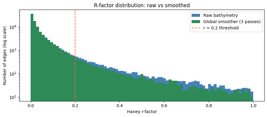
4. Apply the Global smoother
The GlobalBathymetrySmoother applies a node→centroid→node interpolation pass across the entire mesh. Each pass is equivalent to one step of graph-Laplacian smoothing, gently reducing sharp depth gradients throughout the domain. Increasing passes produces stronger smoothing but progressively erodes bathymetric features — choose the minimum needed to satisfy the r-factor criterion in your area of interest.
[9]:
grid_smooth = copy.deepcopy(grid)

smoother.smooth(grid_smooth)

r_smooth = smoother.r_factor(grid_smooth)

print(f'After {smoother._passes} passes of global smoothing:')
print(f'  Max r-factor:       {r_smooth.max():.4f}')
print(f'  Mean r-factor:      {r_smooth.mean():.4f}')
print(f'  Edges with r > 0.2: {(r_smooth > 0.2).sum():,}')
print()
dh = grid_smooth.bathy_nodes - grid.bathy_nodes
print(f'Depth change at nodes:')
print(f'  Max absolute change: {np.abs(dh).max():.3f} m')
print(f'  Nodes modified:      {(np.abs(dh) > 1e-10).sum():,} of {grid.n_nodes:,}')
After 3 passes of global smoothing:
  Max r-factor:       nan
  Mean r-factor:      nan
  Edges with r > 0.2: 5,380

Depth change at nodes:
  Max absolute change: 17.829 m
  Nodes modified:      39,839 of 39,910
5. Comparison plots
[10]:
fig, ax = plt.subplots(figsize=(9, 4))

bins = np.linspace(0, max(np.nanmax(r_raw), np.nanmax(r_smooth)), 80)

ax.hist(r_raw,    bins=bins, label='Raw bathymetry',                        color='steelblue',  log=True)
ax.hist(r_smooth, bins=bins, label=f'Global smoother ({smoother._passes} passes)', color='seagreen',   log=True)
ax.axvline(0.2, color='tomato', linestyle='--', linewidth=1.5, label='r = 0.2 threshold')
ax.set_xlabel('Haney r-factor')
ax.set_ylabel('Number of edges (log scale)')
ax.set_title('R-factor distribution: raw vs smoothed')
ax.legend()
plt.tight_layout()
plt.show()
[11]:
triang = mtri.Triangulation(grid.lon_nodes, grid.lat_nodes, grid.triangles)

fig, axes = plt.subplots(1, 2, figsize=(14, 5), sharex=True, sharey=True,
                         constrained_layout=True)

vmin = min(grid.bathy_nodes.min(), grid_smooth.bathy_nodes.min())
vmax = max(grid.bathy_nodes.max(), grid_smooth.bathy_nodes.max())

for ax, g, title in zip(
    axes,
    [grid, grid_smooth],
    ['Raw bathymetry', f'Global smoother ({smoother._passes} passes)'],
):
    tcf = ax.tricontourf(triang, g.bathy_nodes, levels=50, vmin=vmin, vmax=vmax, cmap='Blues')
    ax.set_title(title)
    ax.set_xlabel('Longitude')
    ax.set_aspect('equal')

axes[0].set_ylabel('Latitude')
fig.colorbar(tcf, ax=axes.tolist(), label='Depth (m)', shrink=0.85)
fig.suptitle('Tamar estuary bathymetry')
plt.show()
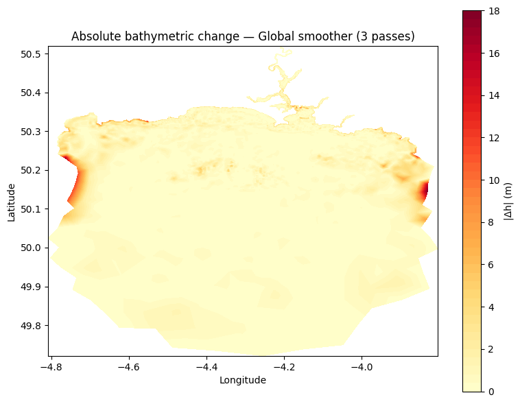
[12]:
dh_abs = np.abs(grid_smooth.bathy_nodes - grid.bathy_nodes)

fig, ax = plt.subplots(figsize=(8, 6))

tcf = ax.tricontourf(triang, dh_abs, levels=50, vmin=0, cmap='YlOrRd')
ax.set_title(f'Absolute bathymetric change — Global smoother ({smoother._passes} passes)')
ax.set_xlabel('Longitude')
ax.set_ylabel('Latitude')
ax.set_aspect('equal')
fig.colorbar(tcf, ax=ax, label='|Δh| (m)')
plt.tight_layout()
plt.show()
6. Write the smoothed grid
Once satisfied with the smoothing, write the modified grid to file. This produces the .dat files consumed by FVCOM’s GRID_FILE and DEPTH_FILE namelist entries.
[13]:
out_dir = os.path.join(data_dir, 'smoothed_inputs')
os.makedirs(out_dir, exist_ok=True)

out_grid  = os.path.join(out_dir, 'tamar_v2_smooth_grd.dat')
out_depth = os.path.join(out_dir, 'tamar_v2_smooth_dep.dat')

grid_smooth.write_grid(
    grid_file=out_grid,
    coordinate_system='geographic',
    depth_file=out_depth,
)

print(f'Smoothed grid written to:  {out_grid}')
print(f'Smoothed depth written to: {out_depth}')
Smoothed grid written to:  /users/modellers/jcl/data/pyfvcom2_doc/FVCOM_tamar_estuary/smoothed_inputs/tamar_v2_smooth_grd.dat
Smoothed depth written to: /users/modellers/jcl/data/pyfvcom2_doc/FVCOM_tamar_estuary/smoothed_inputs/tamar_v2_smooth_dep.dat