Reading and Interpolating TPXO Tidal Harmonics

This tutorial demonstrates how to read TPXO tidal harmonics data and interpolate it onto a target grid using PyFVCOM2. This is useful for:

• Generating tidal boundary forcing for FVCOM from TPXO global tidal models

• Inspecting tidal constituent amplitudes and phases on your model domain

• Comparing TPXO tidal predictions with observations or other models

Overview

TPXO provides global tidal harmonic data on a regular longitude/latitude grid. The data is stored as amplitude and phase (or real/imaginary components) for each tidal constituent. To use this data with FVCOM, we need to interpolate it onto the FVCOM grid or open boundary nodes.

The key steps are:

1. Load TPXO harmonics using TPXOHarmonicsReader

2. Define target interpolation coordinates

3. Use TPXOInterpolator to interpolate harmonics onto the target positions

4. Visualise the interpolated amplitude and phase fields

A note on phase interpolation

Directly interpolating tidal phase is problematic because of the discontinuity at 360°/0°. TPXOInterpolator handles this by decomposing each constituent’s amplitude and phase into two cartesian components using pol2cart, interpolating these smooth fields independently, and then converting back to amplitude and phase with cart2pol.

Prerequisites

Before running this tutorial, ensure you have:

• TPXO harmonics files in NetCDF format (here we use TPXO9.v1)

• The PyFVCOM2 package installed

• Cartopy installed (for map projections in the plots)

Step 1: Import Required Libraries

from collections import namedtuple
import pathlib
import os
import numpy as np
from glob import glob
import matplotlib.pyplot as plt
import cartopy.crs as ccrs
import cartopy.feature as cfeature

from pyfvcom2.fvcom_reader import FVCOMReader
from pyfvcom2.interpolation import InterpolationCoordinates, TPXOInterpolator
from pyfvcom2.tide_reader import TPXOComplexHarmonicsReader, get_tpxo_complex_harmonics_names
from pyfvcom2.plotting import create_figure

/local1/data/scratch/jcl/miniconda/miniconda3/envs/pyfvcom2/lib/python3.11/site-packages/numpy/lib/_format_impl.py:838: VisibleDeprecationWarning: dtype(): align should be passed as Python or NumPy boolean but got `align=0`. Did you mean to pass a tuple to create a subarray type? (Deprecated NumPy 2.4)
  array = pickle.load(fp, **pickle_kwargs)

Step 2: Define the Target Grid

We reuse the same FVCOM domain as in the interpolate_fvcom_data tutorial to define the target grid. The grid limits are taken from the FVCOM mesh, and we create a regular longitude/latitude grid spanning the domain.

# Load FVCOM grid to get domain limits
data_dir = os.path.expanduser('~/data/pyfvcom2_doc')
fvcom_data_dir = f'{data_dir}/FVCOM_tamar_estuary'
fvcom_file_stem = 'fvcom_tamar_estuary_000'
fvcom_file_list = sorted(glob(f'{fvcom_data_dir}/{fvcom_file_stem}*.nc'))
fvcom_reader = FVCOMReader(fvcom_file_list)

# Named tuple for the grid limits
GridLims = namedtuple('GridLims', ('lon_min', 'lon_max', 'lat_min', 'lat_max'))


def get_lons_lats(grid_lims, points_per_degree):
    """Generate 1D lon and lat arrays for a regular grid."""
    n_lon = int((grid_lims.lon_max - grid_lims.lon_min) * points_per_degree)
    n_lat = int((grid_lims.lat_max - grid_lims.lat_min) * points_per_degree)
    lon = np.linspace(grid_lims.lon_min, grid_lims.lon_max, n_lon, dtype=float)
    lat = np.linspace(grid_lims.lat_min, grid_lims.lat_max, n_lat, dtype=float)
    return lon, lat


# Get grid limits from the FVCOM mesh
grid_lims = GridLims(
    fvcom_reader.lon_nodes.min(),
    fvcom_reader.lon_nodes.max(),
    fvcom_reader.lat_nodes.min(),
    fvcom_reader.lat_nodes.max(),
)

# Grid resolution
points_per_degree = 72

# Generate the regular grid
lon, lat = get_lons_lats(grid_lims, points_per_degree)
lon_2D, lat_2D = np.meshgrid(lon, lat, indexing='ij')
lon_flat = lon_2D.flatten()
lat_flat = lat_2D.flatten()

print(f'Domain: {grid_lims}')
print(f'Number of horizontal interpolation points: {lon_flat.size}')

# Create a bounding box for subsetting TPXO global data
bbox = (grid_lims.lon_min, grid_lims.lon_max, grid_lims.lat_min, grid_lims.lat_max)

Accessing FVCOM metadata from: /users/modellers/jcl/data/pyfvcom2_doc/FVCOM_tamar_estuary/fvcom_tamar_estuary_0001.nc
Domain: GridLims(lon_min=np.float32(-4.8078494), lon_max=np.float32(-3.804414), lat_min=np.float32(49.72116), lat_max=np.float32(50.519005))
Number of horizontal interpolation points: 4104

Step 3: Create Interpolation Coordinates

Bundle the target positions into an InterpolationCoordinates object. For tidal harmonics we only need horizontal coordinates — there is no time or depth dimension.

interp_coords = InterpolationCoordinates(
    dates=None,
    x3=None,
    x1=lon_flat,
    x2=lat_flat,
    horizontal_coordinate_system='geographic',
    vertical_coordinate_system='z',
)

Step 4: Read and Interpolate Elevation Harmonics (zeta)

We use TPXOHarmonicsReader to load the tidal elevation harmonics from the TPXO9 file, then use TPXOInterpolator to interpolate them onto our target grid.

The get_tpxo_harmonics_names helper returns the correct variable names for the TPXO amplitude/phase format. For zeta, these are ha (amplitude) and hp (phase).

The TPXO file uses 0–360° longitudes, while the FVCOM domain uses negative longitudes (~-4°). TPXOInterpolator detects and corrects this mismatch automatically.

# Constituent list
constituents = ['M2', 'S2', 'K1', 'O1']

# TPXO files
tpxo_h_files = {}
for c in constituents:
    tpxo_h_files[c] = f'{data_dir}/TPXO/DATA/Atlas10v2/h_{c.lower()}_tpxo10_atlas_30_v2.nc'

# Read harmonics
h_reader = TPXOComplexHarmonicsReader(tpxo_h_files)
h_var_names = get_tpxo_complex_harmonics_names('zeta')
h_harmonics = h_reader.read_harmonics(constituents, h_var_names, fill_land=False, bbox=bbox, bbox_margin=0.1)

print(f'Loaded constituents: {h_harmonics.constituents}')
print(f'Amplitude shape: {np.asarray(h_harmonics.amplitudes).shape}')

# Interpolate onto target grid
h_interpolator = TPXOInterpolator(h_harmonics)
h_result = h_interpolator.interpolate(interp_coords)

print(f'Interpolated amplitude shape: {h_result.amplitudes.shape}')  # (n_points, n_constituents)

Loaded constituents: ['M2', 'S2', 'K1', 'O1']
Amplitude shape: (4, 36, 30)
Interpolated amplitude shape: (4104, 4)

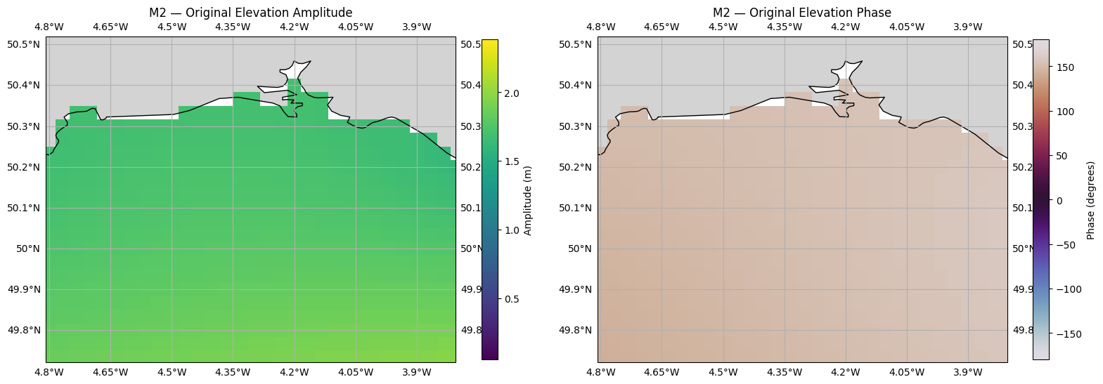
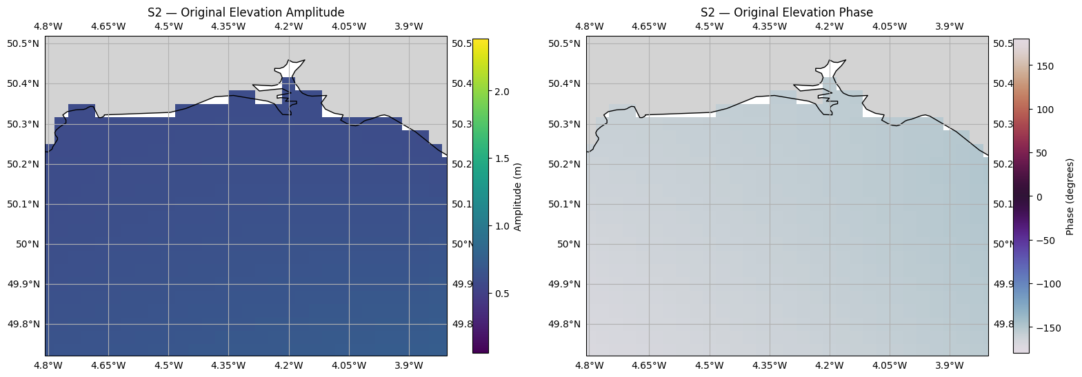
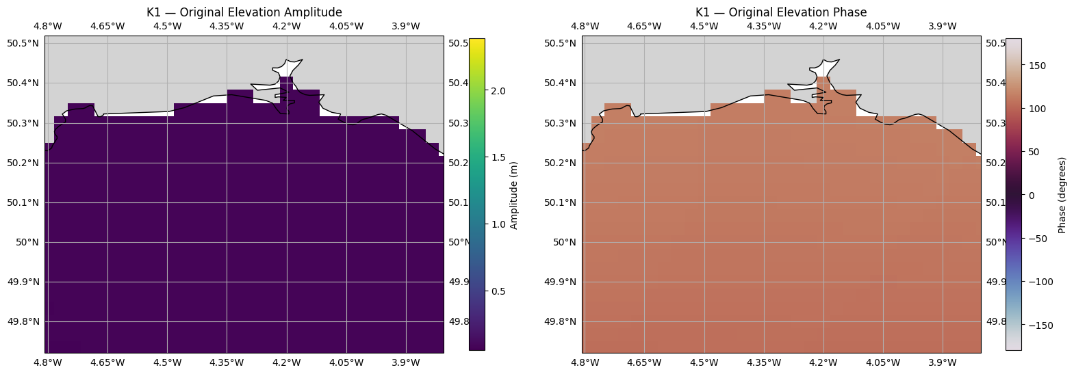
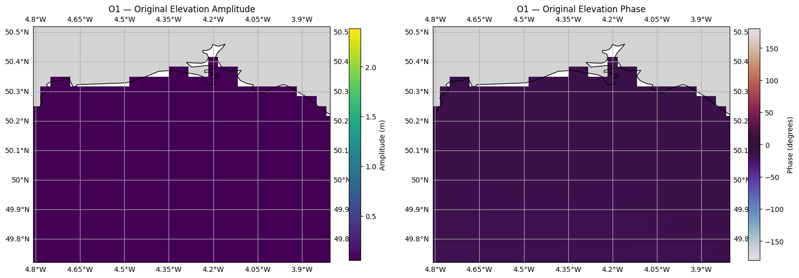
Step 5a: Plot Original (Uninterpolated) Elevation Data

Before looking at the interpolated result, let’s visualise the raw TPXO elevation harmonics over the same domain. The TPXO grid uses 0–360° longitudes, so we shift values > 180° to negative before subsetting to the domain extent.

extent = [grid_lims.lon_min, grid_lims.lon_max, grid_lims.lat_min, grid_lims.lat_max]

# Prepare the raw TPXO elevation grid for plotting
h_lon = np.asarray(h_harmonics.longitude)
h_lat = np.asarray(h_harmonics.latitude)

h_lon_sub_2d, h_lat_sub_2d = np.meshgrid(h_lon, h_lat, indexing='ij')

h_amp = np.asarray(h_harmonics.amplitudes)  # (nc, nx, ny)
h_phase = np.asarray(h_harmonics.phases)

# Compute shared colorbar limits across all constituents for original and interpolated
h_amp_vmin = np.nanmin(h_amp)
h_amp_vmax = np.nanmax(h_amp)

for c_idx, constituent in enumerate(h_harmonics.constituents):
    fig, axes = plt.subplots(1, 2, figsize=(16, 6),
                             subplot_kw={'projection': ccrs.PlateCarree()})

    # Amplitude
    pc = axes[0].pcolormesh(h_lon_sub_2d, h_lat_sub_2d, h_amp[c_idx],
                            cmap='viridis', transform=ccrs.PlateCarree(), shading='auto',
                            vmin=h_amp_vmin, vmax=h_amp_vmax)
    axes[0].coastlines(resolution='10m')
    axes[0].add_feature(cfeature.LAND, facecolor='lightgrey')
    axes[0].gridlines(draw_labels=True)
    axes[0].set_extent(extent, crs=ccrs.PlateCarree())
    cbar = plt.colorbar(pc, ax=axes[0], shrink=0.8)
    cbar.set_label('Amplitude (m)')
    axes[0].set_title(f'{constituent} — Original Elevation Amplitude')

    # Phase
    pc = axes[1].pcolormesh(h_lon_sub_2d, h_lat_sub_2d, h_phase[c_idx],
                            cmap='twilight', transform=ccrs.PlateCarree(), shading='auto',
                            vmin=-180, vmax=180)
    axes[1].coastlines(resolution='10m')
    axes[1].add_feature(cfeature.LAND, facecolor='lightgrey')
    axes[1].gridlines(draw_labels=True)
    axes[1].set_extent(extent, crs=ccrs.PlateCarree())
    cbar = plt.colorbar(pc, ax=axes[1], shrink=0.8)
    cbar.set_label('Phase (degrees)')
    axes[1].set_title(f'{constituent} — Original Elevation Phase')

    plt.tight_layout()
    plt.show()

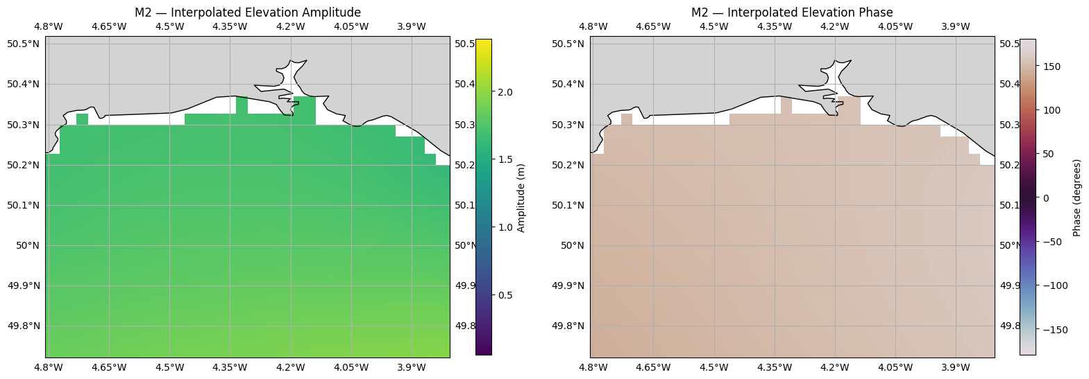
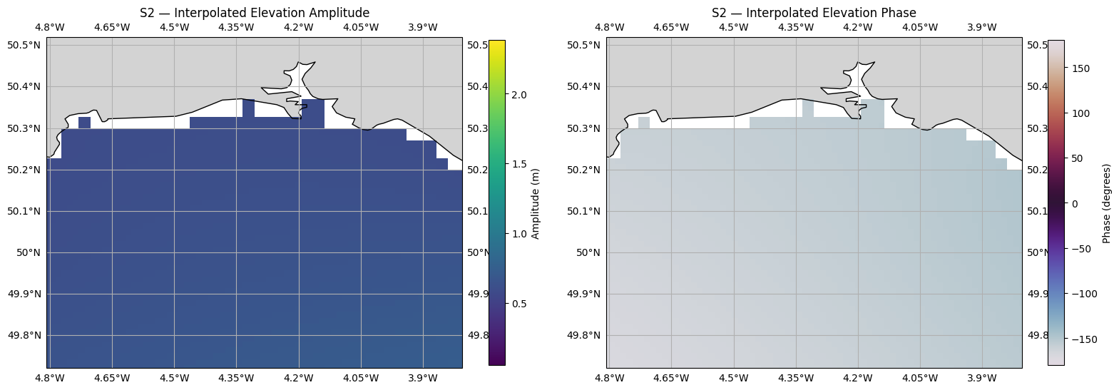
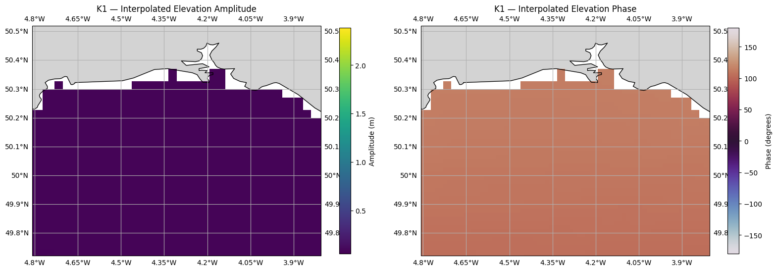
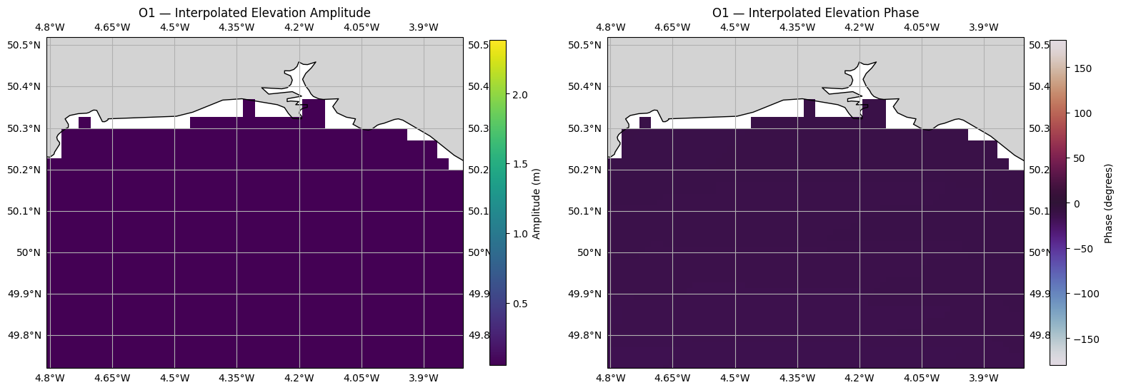
Step 5b: Plot Interpolated Elevation Amplitude and Phase

Plot the interpolated tidal amplitude and phase for each constituent.

n_lon, n_lat = lon_2D.shape

for c_idx, constituent in enumerate(h_result.constituents):
    fig, axes = plt.subplots(1, 2, figsize=(16, 6),
                             subplot_kw={'projection': ccrs.PlateCarree()})

    # Reshape flat interpolated data back to 2D grid
    amp_2d = h_result.amplitudes[:, c_idx].reshape(n_lon, n_lat)
    phase_2d = h_result.phases[:, c_idx].reshape(n_lon, n_lat)

    # Amplitude
    pc = axes[0].pcolormesh(lon_2D, lat_2D, amp_2d, cmap='viridis',
                            transform=ccrs.PlateCarree(), shading='auto',
                            vmin=h_amp_vmin, vmax=h_amp_vmax)
    axes[0].coastlines(resolution='10m')
    axes[0].add_feature(cfeature.LAND, facecolor='lightgrey')
    axes[0].gridlines(draw_labels=True)
    axes[0].set_extent(extent, crs=ccrs.PlateCarree())
    cbar = plt.colorbar(pc, ax=axes[0], shrink=0.8)
    cbar.set_label('Amplitude (m)')
    axes[0].set_title(f'{constituent} — Interpolated Elevation Amplitude')

    # Phase
    pc = axes[1].pcolormesh(lon_2D, lat_2D, phase_2d, cmap='twilight',
                            transform=ccrs.PlateCarree(), shading='auto',
                            vmin=-180, vmax=180)
    axes[1].coastlines(resolution='10m')
    axes[1].add_feature(cfeature.LAND, facecolor='lightgrey')
    axes[1].gridlines(draw_labels=True)
    axes[1].set_extent(extent, crs=ccrs.PlateCarree())
    cbar = plt.colorbar(pc, ax=axes[1], shrink=0.8)
    cbar.set_label('Phase (degrees)')
    axes[1].set_title(f'{constituent} — Interpolated Elevation Phase')

    plt.tight_layout()
    plt.show()

Step 6: Read and Interpolate Velocity Harmonics (u and v)

The TPXO velocity file contains both u (west-east) and v (south-north) components, each on their own grid (lon_u/lat_u and lon_v/lat_v). We read and interpolate them separately.

Note: TPXO9 velocity amplitudes are in cm/s.

# Bathy file
bathy_file = f'{data_dir}/TPXO/DATA/Atlas10v2/grid_tpxo10atlas_v2.nc'

# TPXO files
tpxo_u_files = {}
for c in constituents:
    tpxo_u_files[c] = f'{data_dir}/TPXO/DATA/Atlas10v2/u_{c.lower()}_tpxo10_atlas_30_v2.nc'

# Read harmonics
u_reader = TPXOComplexHarmonicsReader(tpxo_u_files)
u_var_names = get_tpxo_complex_harmonics_names('u')
u_harmonics = u_reader.read_harmonics(constituents, u_var_names, fill_land=False, bbox=bbox, bbox_margin=0.1, bathy_file=bathy_file)

# Read v-component harmonics
v_reader = TPXOComplexHarmonicsReader(tpxo_u_files)
v_var_names = get_tpxo_complex_harmonics_names('v')
v_harmonics = v_reader.read_harmonics(constituents, v_var_names, fill_land=False, bbox=bbox, bbox_margin=0.1, bathy_file=bathy_file)

print(f'u amplitude shape: {np.asarray(u_harmonics.amplitudes).shape}')
print(f'v amplitude shape: {np.asarray(v_harmonics.amplitudes).shape}')

# Interpolate both components onto the target grid
u_interpolator = TPXOInterpolator(u_harmonics, interp_method='nearest')
u_result = u_interpolator.interpolate(interp_coords)

v_interpolator = TPXOInterpolator(v_harmonics, interp_method='nearest')
v_result = v_interpolator.interpolate(interp_coords)

print(f'Interpolated u amplitude shape: {u_result.amplitudes.shape}')
print(f'Interpolated v amplitude shape: {v_result.amplitudes.shape}')

u amplitude shape: (4, 36, 30)
v amplitude shape: (4, 36, 30)
Interpolated u amplitude shape: (4104, 4)
Interpolated v amplitude shape: (4104, 4)

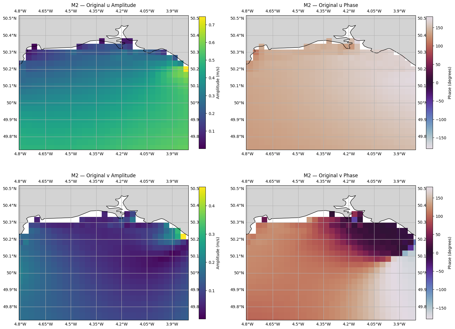
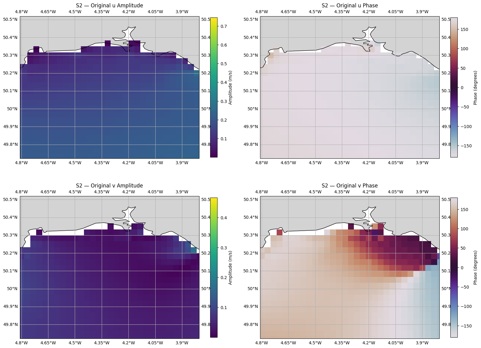
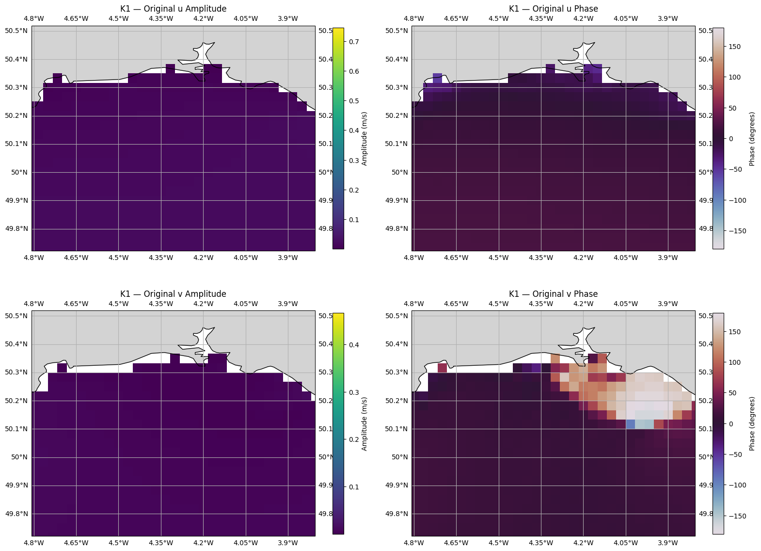
Step 7a: Plot Original (Uninterpolated) Velocity Data

The raw TPXO velocity harmonics for u and v, subset to the same domain.

# Prepare the raw TPXO velocity grids for plotting
u_lon = np.asarray(u_harmonics.longitude)
u_lat = np.asarray(u_harmonics.latitude)
u_lon_2d, u_lat_2d = np.meshgrid(u_lon, u_lat, indexing='ij')
v_lon = np.asarray(v_harmonics.longitude)
v_lat = np.asarray(v_harmonics.latitude)
v_lon_2d, v_lat_2d = np.meshgrid(v_lon, v_lat, indexing='ij')

u_amp = np.asarray(u_harmonics.amplitudes)  # (nc, nx, ny)
u_phase = np.asarray(u_harmonics.phases)
v_amp = np.asarray(v_harmonics.amplitudes)  # (nc, nx, ny)
v_phase = np.asarray(v_harmonics.phases)

# Compute shared colorbar limits across all constituents for original and interpolated
u_amp_vmin = np.nanmin(u_amp)
u_amp_vmax = np.nanmax(u_amp)
v_amp_vmin = np.nanmin(v_amp)
v_amp_vmax = np.nanmax(v_amp)

for c_idx, constituent in enumerate(constituents):
    fig, axes = plt.subplots(2, 2, figsize=(16, 12),
                             subplot_kw={'projection': ccrs.PlateCarree()})

    # u amplitude
    pc = axes[0, 0].pcolormesh(u_lon_2d, u_lat_2d, u_amp[c_idx],
                               cmap='viridis', transform=ccrs.PlateCarree(), shading='auto',
                               vmin=u_amp_vmin, vmax=u_amp_vmax)
    axes[0, 0].coastlines(resolution='10m')
    axes[0, 0].add_feature(cfeature.LAND, facecolor='lightgrey')
    axes[0, 0].gridlines(draw_labels=True)
    axes[0, 0].set_extent(extent, crs=ccrs.PlateCarree())
    cbar = plt.colorbar(pc, ax=axes[0, 0], shrink=0.8)
    cbar.set_label('Amplitude (m/s)')
    axes[0, 0].set_title(f'{constituent} — Original u Amplitude')

    # u phase
    pc = axes[0, 1].pcolormesh(u_lon_2d, u_lat_2d, u_phase[c_idx],
                               cmap='twilight', transform=ccrs.PlateCarree(), shading='auto',
                               vmin=-180, vmax=180)
    axes[0, 1].coastlines(resolution='10m')
    axes[0, 1].add_feature(cfeature.LAND, facecolor='lightgrey')
    axes[0, 1].gridlines(draw_labels=True)
    axes[0, 1].set_extent(extent, crs=ccrs.PlateCarree())
    cbar = plt.colorbar(pc, ax=axes[0, 1], shrink=0.8)
    cbar.set_label('Phase (degrees)')
    axes[0, 1].set_title(f'{constituent} — Original u Phase')

    # v amplitude
    pc = axes[1, 0].pcolormesh(v_lon_2d, v_lat_2d, v_amp[c_idx],
                               cmap='viridis', transform=ccrs.PlateCarree(), shading='auto',
                               vmin=v_amp_vmin, vmax=v_amp_vmax)
    axes[1, 0].coastlines(resolution='10m')
    axes[1, 0].add_feature(cfeature.LAND, facecolor='lightgrey')
    axes[1, 0].gridlines(draw_labels=True)
    axes[1, 0].set_extent(extent, crs=ccrs.PlateCarree())
    cbar = plt.colorbar(pc, ax=axes[1, 0], shrink=0.8)
    cbar.set_label('Amplitude (m/s)')
    axes[1, 0].set_title(f'{constituent} — Original v Amplitude')

    # v phase
    pc = axes[1, 1].pcolormesh(v_lon_2d, v_lat_2d, v_phase[c_idx],
                               cmap='twilight', transform=ccrs.PlateCarree(), shading='auto',
                               vmin=-180, vmax=180)
    axes[1, 1].coastlines(resolution='10m')
    axes[1, 1].add_feature(cfeature.LAND, facecolor='lightgrey')
    axes[1, 1].gridlines(draw_labels=True)
    axes[1, 1].set_extent(extent, crs=ccrs.PlateCarree())
    cbar = plt.colorbar(pc, ax=axes[1, 1], shrink=0.8)
    cbar.set_label('Phase (degrees)')
    axes[1, 1].set_title(f'{constituent} — Original v Phase')

    plt.tight_layout()
    plt.show()

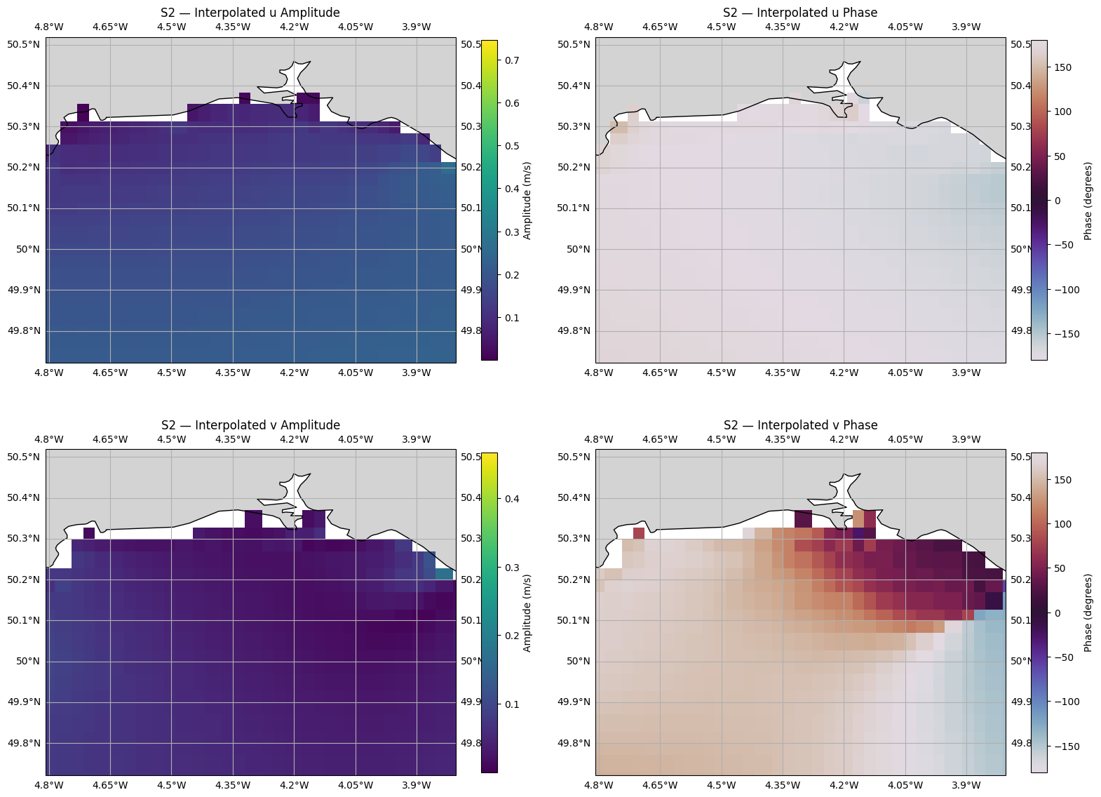
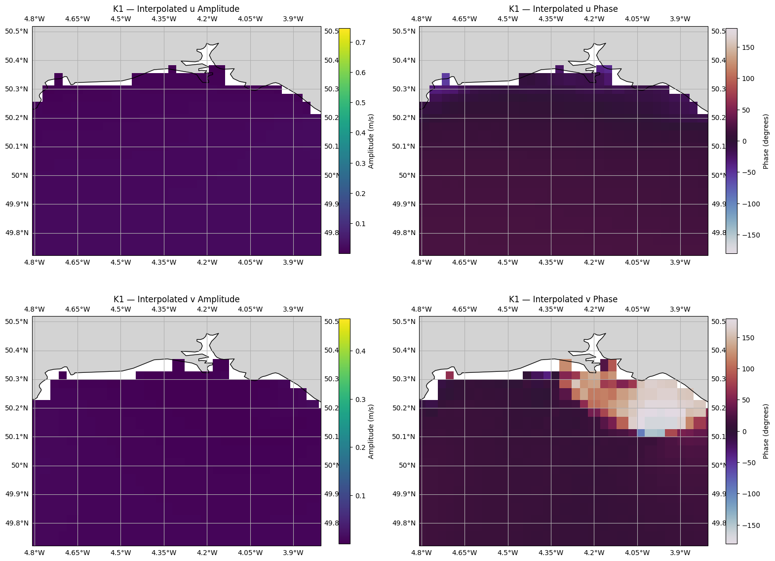
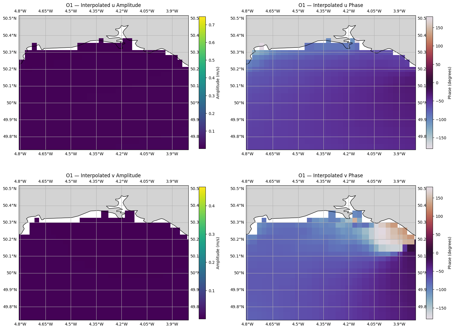
Step 7b: Plot Interpolated Velocity Amplitude and Phase

Plot the interpolated u and v velocity amplitudes and phases for each constituent.

for c_idx, constituent in enumerate(constituents):
    fig, axes = plt.subplots(2, 2, figsize=(16, 12),
                             subplot_kw={'projection': ccrs.PlateCarree()})

    # Reshape flat interpolated data back to 2D grid
    u_amp_2d = u_result.amplitudes[:, c_idx].reshape(n_lon, n_lat)
    u_phase_2d = u_result.phases[:, c_idx].reshape(n_lon, n_lat)
    v_amp_2d = v_result.amplitudes[:, c_idx].reshape(n_lon, n_lat)
    v_phase_2d = v_result.phases[:, c_idx].reshape(n_lon, n_lat)

    # u amplitude
    pc = axes[0, 0].pcolormesh(lon_2D, lat_2D, u_amp_2d, cmap='viridis',
                               transform=ccrs.PlateCarree(), shading='auto',
                               vmin=u_amp_vmin, vmax=u_amp_vmax)
    axes[0, 0].coastlines(resolution='10m')
    axes[0, 0].add_feature(cfeature.LAND, facecolor='lightgrey')
    axes[0, 0].gridlines(draw_labels=True)
    axes[0, 0].set_extent(extent, crs=ccrs.PlateCarree())
    cbar = plt.colorbar(pc, ax=axes[0, 0], shrink=0.8)
    cbar.set_label('Amplitude (m/s)')
    axes[0, 0].set_title(f'{constituent} — Interpolated u Amplitude')

    # u phase
    pc = axes[0, 1].pcolormesh(lon_2D, lat_2D, u_phase_2d, cmap='twilight',
                               transform=ccrs.PlateCarree(), shading='auto',
                               vmin=-180, vmax=180)
    axes[0, 1].coastlines(resolution='10m')
    axes[0, 1].add_feature(cfeature.LAND, facecolor='lightgrey')
    axes[0, 1].gridlines(draw_labels=True)
    axes[0, 1].set_extent(extent, crs=ccrs.PlateCarree())
    cbar = plt.colorbar(pc, ax=axes[0, 1], shrink=0.8)
    cbar.set_label('Phase (degrees)')
    axes[0, 1].set_title(f'{constituent} — Interpolated u Phase')

    # v amplitude
    pc = axes[1, 0].pcolormesh(lon_2D, lat_2D, v_amp_2d, cmap='viridis',
                               transform=ccrs.PlateCarree(), shading='auto',
                               vmin=v_amp_vmin, vmax=v_amp_vmax)
    axes[1, 0].coastlines(resolution='10m')
    axes[1, 0].add_feature(cfeature.LAND, facecolor='lightgrey')
    axes[1, 0].gridlines(draw_labels=True)
    axes[1, 0].set_extent(extent, crs=ccrs.PlateCarree())
    cbar = plt.colorbar(pc, ax=axes[1, 0], shrink=0.8)
    cbar.set_label('Amplitude (m/s)')
    axes[1, 0].set_title(f'{constituent} — Interpolated v Amplitude')

    # v phase
    pc = axes[1, 1].pcolormesh(lon_2D, lat_2D, v_phase_2d, cmap='twilight',
                               transform=ccrs.PlateCarree(), shading='auto',
                               vmin=-180, vmax=180)
    axes[1, 1].coastlines(resolution='10m')
    axes[1, 1].add_feature(cfeature.LAND, facecolor='lightgrey')
    axes[1, 1].gridlines(draw_labels=True)
    axes[1, 1].set_extent(extent, crs=ccrs.PlateCarree())
    cbar = plt.colorbar(pc, ax=axes[1, 1], shrink=0.8)
    cbar.set_label('Phase (degrees)')
    axes[1, 1].set_title(f'{constituent} — Interpolated v Phase')

    plt.tight_layout()
    plt.show()